Predicting the price of Magic: The Gathering cards after they are reprinted
In this post I’m going to demonstrate how a recurrent neural network can be used to forecast a time-series in response to external stimuli. A real-world application of this type of analysis could be the foreign exchange market responding to, say, a change in interest rates, but here I’ll use the much simpler example of the price of Magic: The Gathering cards after a reprint. I recently got back into playing Magic after about 15 years, and I’m happy that my current more-mathematically minded brain is finding many ways of analysing the game (so expect more posts on this in the near future).
Recurrent neural networks are especially good for sequence prediction tasks, and they’re the go-to model for many language tasks (see The Unreasonable Effectiveness of Recurrent Neural Networks). They are popular methods for character prediction (predictive text). Say you have typed two characters, “th”, a recurrent neural network can be trained to give you the probability that the next character is “e” or another letter. I won’t the workings of this type of neural network here, see here for the details.
Magic: The Gathering
In case you haven’t heard of it before, Magic: The Gathering (Magic or MTG for short) is a trading card game developed by Wizards of the Coast. As card games go it’s pretty complicated, but the jist is that you and your opponent take turns to wittle each others’ life down from 20 to 0. It’s interesting for a few reasons: you typically build your own deck based around some strategy, and so you need to think about the probabilities of drawing certain cards in a game (there are also cards that exist purely to manipulate the probability of drawing a certain card). Typically your deck may contain 60+ cards, with a maximum of 4 copies of any one card (except for basic land cards, which are unlimited). To increase the chances of drawing key cards during play it’s most common to have exactly 60 cards and run 4 copies of important cards.
The cards enter circulation via booster packs, which are a sealed back of 15 randomly selected cards consisting of 1 rare , 3 uncommons and 11 common cards. Sometimes the rare is replaced with a mythic rare, and in every booster pack one of the cards is printed on shiny foil rather than paper. Remarkably this has led to a very large secondary market where people buy and sell the individual cards on ebay.com and tcgplayer.com), and there are websites such as mtgstocks.com to track the prices over time.
 Image author Tourtefouille (wikimedia commons).
Supply and demand, of Magic cards
Like most markets, the price of Magic cards on the secondary market is driven by two factors: supply and demand. If a card is rare it’s printed less, and so supply is low. If a card is “good” then lots of people want it, and so demand is high. Here, good means that either the artwork is nice or the card does something amazing in play. Wizards of the Coast don’t just continually print off cards though: they are printed as part of a set, and new sets are released every few months. Old cards (those from old sets that are “out of print”) are often worth more, and their slow rise in value over time can probably be attributed to an a gradual increase in the number of MTG players. Each time Wizards release a new set, they include reprints of older cards and so the price of those cards falls as you’d expect.
This makes for a pretty cool time-series forecasting problem under the influence of external stimuli. Most of the examples I’ve seen online of time-series forecasting are autoregressive models, where predictions are made using historical values. Here I’m going to use a neural network to demonostrate how one could try to predict the expected draw-down in the value of a Magic card after its reprinted. Instead of doing this for the real prices of Magic cards I’ll generate some data that looks a lot like actual price data, and see if the neural network is able to model the mechanics.
Recurrent neural network for Time-series
Neural networks are in the news a lot lately due to the huge amount of progress made on deep-learning in the last decade. Here I’ll use a type of recurrent neural network called an LSTM network (LSTM stands for long short term memory) to predict the price of a Magic card one day into the future.
Setting up the data
For now, we’ll just generate some data that mimics the price movements of a typical magic card in response to it being reprinted. This is helpful for two reasons: we can generate as much data as needed to train the network, and we can experiment with the amount of noise in the data. This also simplifies the problem somewhat: as we’re mainly interested to see how well the model can pick up on the effect a reprint has on the price.
Here’s a function to make a time-series of price and reprint status for our fictitious Magic card,
def mkts(length=4001, y0=1.0):
    reprint_log = [1] # card was printed at t0
    y = [y0] # starting price
    t_since_reprint = 0
    for i in range(length-1):
        reprint = 0
        rdev = np.random.rand()

        if rdev > 0.995 and t_since_reprint > 300:
            t_since_reprint = 0
            reprint = 1
        else:
            t_since_reprint += 1

        trend = 0.005
        if t_since_reprint > 0: # price doesn't instantly respond to reprints
            if t_since_reprint < 20:
                trend = -0.007
            elif t_since_reprint < 200:
                trend = -0.002

        reprint_log.append([reprint])
        y.append(y[-1] + trend + np.random.randn()*0.00001)
    return np.array(reprint_log), np.array(y)
Plotting the resulting price time-series (blue line) and the reprint status (green impulses) gives the graph below. Overall the price trends up, but when there’s a reprint the price drops for the following 200 days. It’s important to note that there is no intentional seasonality in the price time-series here. The “card” was reprinted at random intervals (see the mkts() function), and so it will be impossible to predict the resulting price drops with an autoregressive model.
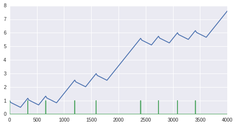 Price (blue) and reprint-status (green).
As we specifically want the model to learn the response to reprints, I’m going to subtract out the overall trend:
gradient = (y[-1] - y[0])/len(y)print 'gradient:',gradient
y = y - gradient * np.arange(len(y))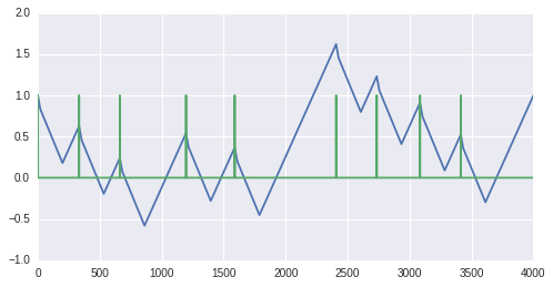 Price with the overall trend substracted (blue) and reprint-status (green).
Next, as we want to predict price change we will use the differential time-series, which
is the difference between the current price and the previous one (sometimes called returns),
and standardize the data to speed up training of the network.
This is standard pracitce, but if you want to see the details of this, see the
Jupyter notebook here.
Setting up the neural network
We do the predictions using a very simple neural network implemented using Keras, which is an excellent Python library for quickly prototyping ideas. It’s really just a wrapper on top of Tensorflow (or Theano if you prefer) but it handles training and data augmentation tasks very elegantly. See the Keras documentation, and also this example, for details.
# batch size of 100 samples, 1 time-step with 2 features...
model = Sequential()
model.add(LSTM(12, batch_input_shape=(100, 1, 2),
               stateful=True, return_sequences=False))
model.add(Dropout(0.25))
model.add(Dense(1)) # just a single output from the network
model.compile(loss='mean_squared_error', optimizer='adam')

# as we're using a stateful LSTM layer, we need to train
# on epoch at a time and reset the cell states between epochs.
nb_epochs = 100
for i in range(nb_epochs):
    model.fit(Xrnn[:-1000], ydiff[:-1000],
              nb_epoch=1, batch_size=100,
              verbose=2, shuffle=False)
    model.reset_states()
This trains in a few seconds, and you should notice the loss decreases each iteration:
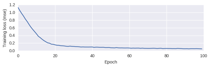 Training loss (mean squared error) vs. epochs.
Testing the model (getting out predictions)
So far we made some data that looks like the daily price time-series for a typical Magic: The Gathering card, as it undergoes several reprints. We then represented this in a form that’s tractable using machine-learning and we just trained a recurrent neural network to predict the next price move (given the last price move and an attribute indicating whether or not the card was reprinted).
From the training loss above, things are looking quite positive, but neural networks can easily overfit to the training data and so we need to see how well our model generalizes to unseen data.
# get predictions for the unseen data
preds = model.predict(Xrnn[-1000:], batch_size=100).flatten()
# reverse the standardization we did above
unscaled_preds = mm.inverse_transform(preds)
shift = y[-1000] # the last y-value (price-value) in the training set
# use cummulative sum to go from the returns-series to the time-series
predicted_prices = np.cumsum(unscaled_preds) + shift
Sanity check. At this point it’s really important to verify one thing: does our neural network have real predictive power, or is it just copying the input value onto the output?! When conducting regression on a continuous time-series the squared loss metric, using the current known value of the price as a guess for the next price is always going to be a pretty reasonable choice. This would lead to a type of trend-following behaviour that only really appears to work because we’re only forecasting a single time-step into the future. Fortunately, the plots (below) show that our simple network is able to correctly predict one step into the future for our (very) simple model!
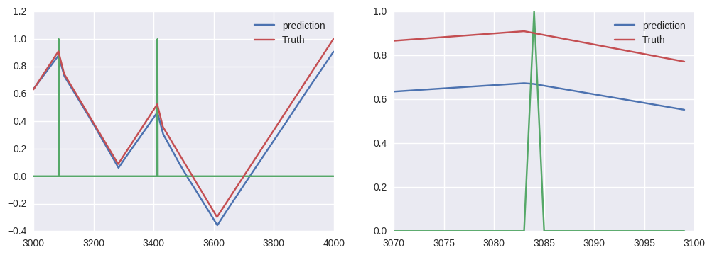 Predictions from our neural network model! The left plot shows predictions over
the whole testing set, while the right plot shows a zoomed in region (to verify
that the predictions aren't just a lagged copy of the input data).
Predictions from our neural network model! The left plot shows predictions over
the whole testing set, while the right plot shows a zoomed in region (to verify
that the predictions aren't just a lagged copy of the input data).
Conclusions
-
We built a model of the price of a ficticious Magic: The Gathering playing card, over time, as it undergoes several reprints (in our simple model, each reprint leads to a small drop in price for the subsequent 200 days).
-
We implemented a small neural network, utilising the LSTM layer to predict these price movements, one day in advance.
-
This is all really simplistic, but it demonstrates how LSTM networks can be used to predict time-series in response to external stimuli. If we were to replace the LSTM layer in our code above with a Keras dense layer (i.e. a fully-connected layer) then the network would fail to predict accurately. This is because LSTM layers are stateful, and information from the previous time-steps is still used to make predictions even though they aren’t provided as features to the current time-step.
-
This model works really well in the absense of significant noise in the price time-series. If we add noise, it just fails to make accurate predictions. This is because the “correct” behaviour after a reprint is sometimes masked in the training data, so the network can’t learn a consistent rule. There are a couple of ways around this - one of the best fixes would just be to predict the next \(N\)-steps (e.g. the next 20 time-steps), as the error signal will be averaged over more samples and the noise has less influence on longer time-scales.