Unsupervised domain adaption by backpropagation: method discussion and implementation
When training deep neural networks (or any machine-learning model) for some task we typcially assume that the distributions of the features for training and test data are the same: that is, if we concatenated the train and test datasets together we shouldn’t be able to build a classifier that will do well at distinguishing them. When the train and test distributions differ we call this domain shift or covariate shift. This distribution shift can happen for various reasons, and is most typically associated with data collected over a long time period due to changes in the underlying system being measured or in the method of measurement. Two textbook examples would be stock market data, where market conditions change over time, or medical data collected over a period of decades.
One approach that’s sometimes used is to re-weight samples in the training set according to their likeness to testing samples [1-2]. Let’s say we have classification function \(f(x)\) that maps features to predicted labels \(X \rightarrow \hat{y}\) and we wanted to compute the expectation value of our loss function \(l(y, \hat{y})\) (for true labels \(y\), where \(l(y, \hat{y})\) could for instance be the crossentropy loss function). The expected loss on the test set is then,
The factor \( \frac{p(X_{test})}{p(X_{train})} \) can be viewed as importance weights, that upweight samples in the training set that look most like sampels in thet test set. To evaluate this weight factor for the training set, we use the property that \( p(X_{train}) + p(X_{test}) = 1 \),
All that is to estimate , which can be done by training a classifier to discriminate between train and test sets. For a really basic example of this, see my Jupyter notebook. Also for a more thorough introduction to this technique see the video lecture here.
Domain adaption by backpropagation
The covariate shift by importance weighting method above is reasonably effective when there is a slight shift in distributions between the training and test data. However it doesn’t help in situations where there is very little (or no) overlap between the training and testing distributions. The approach proposed in [3] (Unsupervised domain adaption by backpropagation, Ganin, Y., & Lempitsky, V. (2014)), aims to help domain adaptive learning by simultaneously training a deep neural network on labelled training data (called “source” data) and unlabelled testing data (called “target” data).
In a neural network each layer transforms the data going into it by some linear transformation (basically multiplying by a matrix of weights) and a nonlinear transformation (called the activation function). During training each layer learns to generate a new representation of the data that’s useful to layers above it until the final layer, which uses the features of the representation generated by the previous layer to output some class prediction \(\hat{y}\in [0,1]\). Neural networks learn to produce better predictions by backpropagation, which uses the partial derivative of the loss function with respect to each individual weight in the network with gradient descent (or similar) to incrementally move the weights in the right direction each iteration. In [3] the authors proposed that by making the learned representations, upon which the final classification layer makes its decisions, invariant between the source and target domains the learned model should be applicable to the target domain. Unlike some earlier methods this does not require labelled samples from the target dataset, although a few labelled target samples could be introduced to speed up learning.
To achieve this the authors designed the network architecture shown in the figure below (taken from their paper). The network looks like a relatively simple multi-output graph, which attempts to simultaneously predict both the class label and the domain (source vs. target) of the input data. Their innovation was to introduce a gradient reversal layer between the the shared feature layer (the last green layer) and the domain classifier, which simply flips the sign on the gradient during backpropagation.
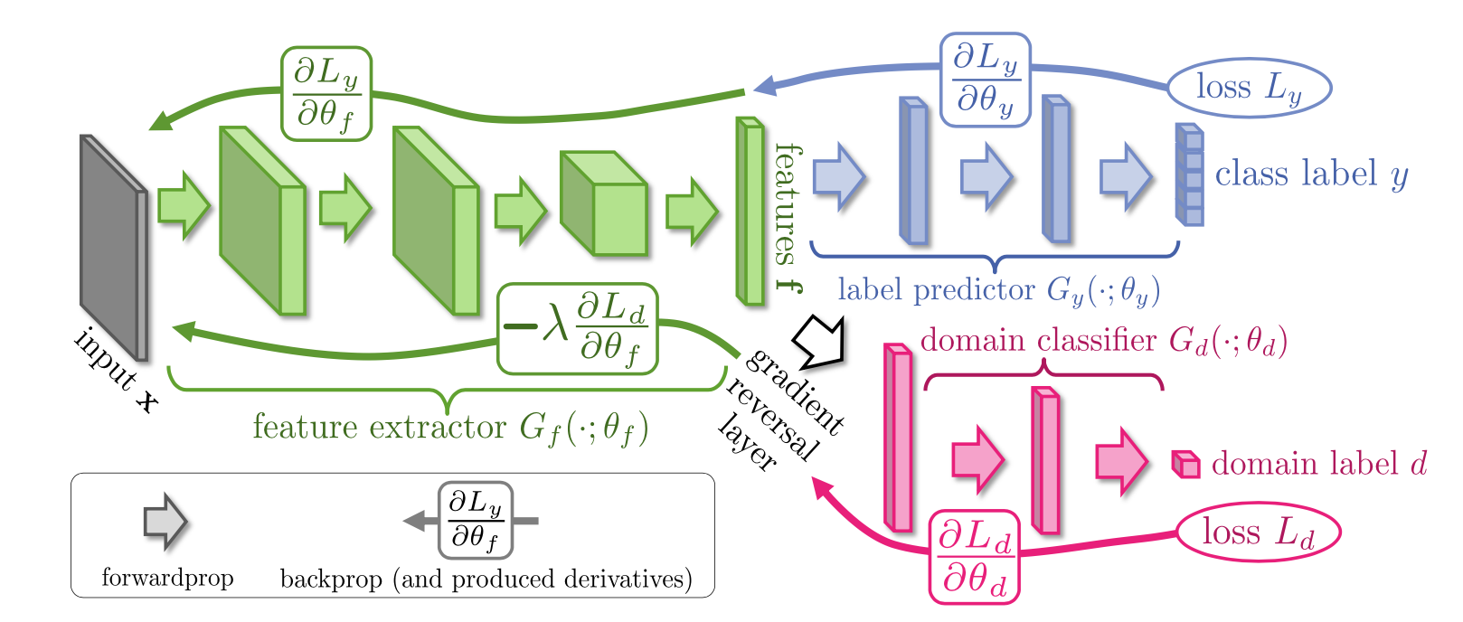 Unsupervised domain-adaption architecture. Image taken from ref. [3].
During backpropagation the weights in each layer are updated according to gradient of the loss function with respect to each weight; this gradient contains the information on which direction to move the weights in to reduce the loss value at each iteration. Without the gradient reversal layer the feature extractor would simply learn to create a representation of the input that was good for both classification of the labels and determining which domain the data came from. The gradient reversal layer forces the network to learn features that are bad for discriminating between the source and target domain. By flipping the sign of the gradient between the start of the domain classifier branch (pink) and the feature representation layer (final green layer) the weights of the feature extractor are shifted so that the domain classifier cannot discriminate between source and target distributions.
Implementation
On the author’s homepage they kindly provide a link to an implementation of this method in Caffe, which was ported to TensorFlow. My own implementation borrows heavily from this TensorFlow version, but wraps the approach up in a class for easier use and talks nicely to TensorBoard for visualisation of the network in your browser. The training proceedure in each case is the same: we create batches consisting of half source data and half target data, with labels for both domain and the class for each sample. As target labels are unknown (this is unsupervised after all) those are not used in training (see here for implementation details).
Testing
How does this perform? The authors of ref. [3] reported very solid performance on some standard datasets. Here I want to show it working on a really simple 2-dimensional problem, which has been taken directly from the original TensorFlow implementation [4].
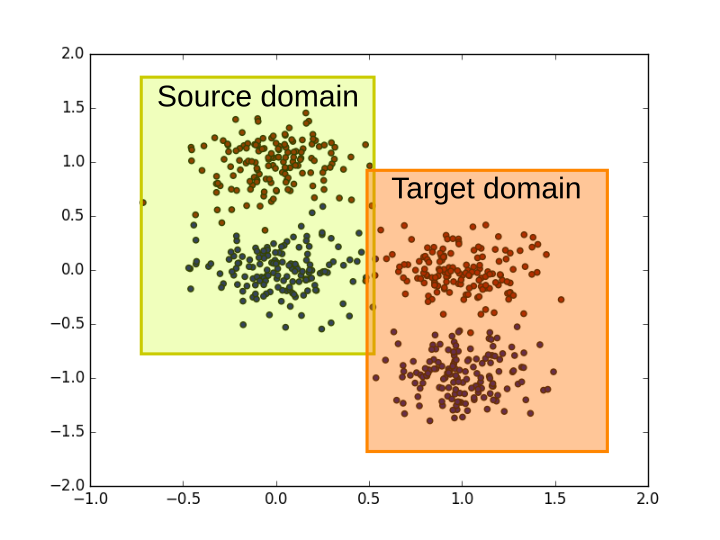 Two blobs, with domain shift between source (train) and target (test). Idea taken from [4].
I made a video of the decision boundary at each training iteration, shown below. First the network learn to separate the two blobs in the labelled source data by making a roughly horizontal line, but completely fails to generalize to the target data. The decision boundary gradually shifts to a diagonal line, which does a good job of classifying both the source and target data.
References
[1] Shimodaira, H. (2000). Improving predictive inference under covariate shift by weighting the log-likelihood function. Journal of Statistical Planning and Inference, 90, 227–244.
[2] Bickel, S. et al. (2009). Discriminative Learning Under Covariate Shift. Journal of Machine Learning Research, 10, 2137-2155
[3] Ganin, Y., and Lempitsky, V. Unsupervised domain adaptation by backpropagation. International Conference on Machine Learning. 2015.
[4] https://github.com/pumpikano/tf-dann