Optimization and sampling methods Part 1: Introducing gradient descent
The problem
Let’s say you have some function \( y(x) = x^2 \), and we want to find the value of \(x\) that minimises \(y\), or more formally,
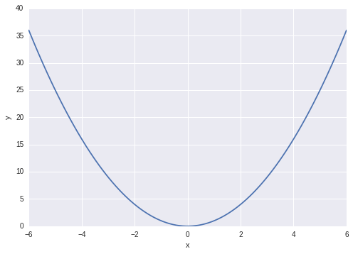
Of course you could just differentiate and find the stationary point(s), then differentiate again to get the curvature to show that it’s a minimum (and not a maximum), and since the above function is convex we know that we’ve got the global minimum. Here we’re not going to do that: we’ll just be using this equation as a model system on which to build some neat concepts that are used for optimization, and sampling from general functions.
Optimization problems are of general importance, e.g. from the principle of a minimum potential energy in physics we know that systems in equilibrium will tend towards their low-energy states. In supervised machine-learning you often construct a loss (or cost) function, which you set about minimising with respect the parameters of the model. We’ll see more about these in later posts, for now let’s just think about \( y(x) = x^2 \).
Gradient Descent
From the definition of differentiation we know that,
The derivative \(y’(x)\) is the tangent of the function \(y(x)\) at \(x\). This tells us that if \(y’(x)\) is positive then \(y(x)\) is sloping upwards, and we can see for \(h\to 0\), if we have \(y’(x) > 0 \) then we know that \(y(x+h) > y(x)\).
Gradient descent (also known as steepest descent) follows directly from this. We can find a local minimum of any (differentiable) function by iteratively taking tiny steps “downhill”, following the direction of the negative of the gradient.
We’ll need to make small but finite steps. To achieve this we’ll use a learning rate, which determines the step size we take with each iteration. The learning rate is often denoted by \(\alpha\) (or sometimes \(\eta\)), and we write the full gradient descent algorithm for a single iteration as,
The learning rate is a tunable parameter (hyperparameter) of the gradient descent method, and it might take a few attempts to find one that converges well. If the learning rate is too small then your system will take many iterations to converge (and you may run into issues with machine precision), if the learning rate is too big then you’ll just diverge away from the solution! It’s common practice in machine learning to anneal the learning rate, by gradually reducing it over time (a similar technique has been used on phyiscal chemistry to find the low-energy conformations of molecules, by gradually reducing the temperature over the course of a simulation).
For those who prefer code to maths, it’s just a few lines of Python:
# Gradient descent to find min of y(x)=x^2
n_iter = 25 # number of iterations
lr = 0.1 # learning rate
x = 4.3 # our starting "guess" for x
for i in range(n_iter):
   # dy/dx = 2*x
   x -= lr*(2*x)
If you run the above code and plot the results each iteration, you’ll get something like this:
 Gradient descent for a simple convex function, showing each iteration of the optimization.
If you look at the animated graphs above you’ll notice that gradient descent takes biggest steps to start with, which is simply because the gradient is larger. You might also notice that even those it gets very, very close to the exact value of zero, it never quite reaches it.
What about multiple local minima?
If you have a differentiable function and you want to find a local minimum (or maximum) you can use gradient descent. Note that I said local minimum because for a potential with multiple local minima gradient descent will only move into whichever is closest to its starting point. Here we didn’t have this problem, as the function we’ve been working with is convex (and so the local minimum is also the global minimum). In the real world things are harder, and we often have to work with non-convex systems sometimes with a very large number of local minima! Consider the following 1-d function,
 Gradient descent with random starting positions. Optimization moves to the nearest local minimum.
There are two local minima at \(\pm 3\), but the one minima at \(-3\) is slightly lower. If we started from say \(x=-1\) we would reach the global minimum, but if we started from a value of \(x\) greater than zero we’d end converging to the local minima at \(x=3\). This is actually a general problem, bridging physics, molecular simulation and machine learning, to which there exists no generally superior solution. There are multiple methods in each of these disciplines to cope with this issue, for example simulated annealing, metadynamics, and multiple random starts.
What next?
In part 2 I’ll connect the above to some simple physics, and make the connection between gradient descent and molecular dynamics. In parts 3 and 4 I’ll talk about higher-order methods (leapfrog and velocity Verlet) and finally how Markov-chain Monte Carlo methods (Metropolis and hybrid/Hamiltonian Monte Carlo) can be used to sample a posterior distribution.