Optimization and sampling methods Part 2: The harmonic oscillator

The harmonic oscillator

In part 1 we introduced gradient descent and used it to optimize a simple 1-d equation,

$y(x) = x^2.$

While this is a pretty simple problem, it actually describes an incredibly important physical model: the harmonic oscillator (i.e. a spring). It’s important because it’s one of the few problems in physics we can actually solve exactly, and it turns out that even anharmonic functions are approximately harmonic near their minimum.

The potential energy of a harmonic oscillator with spring-constant $k$ is $V(x) = \frac{1}{2}k x^2$, and the force on it is $F(x) = -\frac{dV}{dx} = -k x$ (Hook’s Law). Note the similarities with gradient descent, it turns out we actually found the minimum of a harmonic oscillator with $k=2$, and the derivative (slope) in gradient descent corresponds to the force! To be consistent with the previous part we’ll work with $k=2$ for the rest of this article.

Molecular dynamics

Since we are now considering a physical system we can do more than just find the minimum state: we can see how it evolves with time. To do this, we need just a little bit more physics: the principle of conservation of total energy. This means that when the harmonic oscillator moves to a state with lower potential energy $V$, it gains some kinetic energy $T$ equal to the amount of potential energy it lost. If $E$ is the total energy then we can write this as,

$E = T + V.$

Note that $T$ in the above equation is not really the temperature, and I say not really because on some level kinetic energy is very closely related to temperature, but that’s beyond the scope of this article.

We’ll introduce one more thing from physics: time. In the previous article $x$ was the free parameter, but here $x(t)$ will be the position of our oscillator at time $t$.

Euler method

Let’s say we know at some time $t$ we know the position of our spring and so by the above equations we know its potential energy and the force acting on it. If we wanted to know the position at some future time $t + \Delta t$, we can first do a Taylor expansion,

$x(t+\Delta t) = x(t) + \Delta t \frac{dx(t)}{dt} + O(\Delta t^2).$

Then by recognising that the first and second derivatives of x(t) are the velocity and acceleration respectively, we have,

$v(t + \frac{\Delta t}{2}) = v(t - \frac{\Delta t}{2}) + \frac{F(t)}{m}\Delta t,$

which we can then plug into the expression for the position update,

$x(t + \Delta t) = x(t) + v(t+\frac{\Delta t}{2})\Delta t.$

We normally assume that $ v(0) = 0 $, and so the very first velocity step is actually a half-step in time, i.e.,

$v(0 + \frac{\Delta t}{2}) = v(0) + \frac{F(0)}{2m}\Delta t.$

The Euler method then consists of iteratively applying the equations above to propagate the system forward in time. Note that it’s basically just the gradient descent method we derived in part 1 (here we are working in time, while there we were using $x$ as the independent variable). In the previous section we derived gradient descent from the definition of differentiation, and here we used a Taylor series. Deriving these integrators using a Taylor series is useful because it’s very clear where you are truncating the series and therefore what the error in each step is. Note that in the Euler method the step-error is $O(\Delta t^2)$, however since a trajectory involves ((N)) steps of size $\Delta t = 1/N$ then the total error is of the order $\Delta t$. In part 3 we’ll use the Taylor series to find more accurate, higher-order methods!

Code

Here’s the code, in Python:

# Euler integration of harmonic oscillator V(x) = x^2 with mass = 1
n_iter = 10000 # number of iterations
dt = 0.001 # step size
x = 4.3 # our starting position x(0)

# first we need to calculate the v(0+1/2t) term
v_old = -x*dt

# save these for plotting
trajectory = []
velocities = []

# do the iterations
for i in range(n_iter):
    
    v_next = v_old - 2*x*dt
    x_next = x + v_next*dt

    trajectory.append(x_next)
    velocities.append(0.5*(v_next + v_old))
    
    x = x_next # new becomes old
    v_old = v_next

After running the above code we can generate the plots below, showing the position and the velocity at each time-step of the simulation. Notice that the velocity goes through zero whenever the harmonic oscillator changes direction, which is as we’d expect. Also the oscillator is approximately bound between $ \pm x_0 $ (where $ x_0 = x(0) = 4.3 $. This is important, if the time-step was too large our oscillator would reach values of $x$ that are unphysical (much like how we saw that gradient descent could diverge for a large learning-rate).

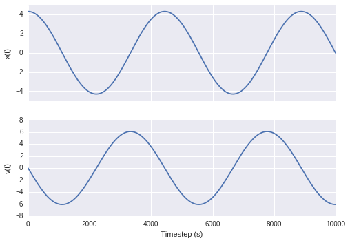Plotting the position and velocity at each time-step for the Euler integration above.

Phase space representation

It’s pretty clear from the figure above that both the position ($x(t)$) and the velocity ($v(t)$) are oscillating, and that they are linked. In fact, it turns out the potential energy $V$ depends only on the position, while the kinetic energy depends only on the velocity, and as a result it’s more common to represent the above graphs on a single plot that we cell phase space. For our harmonic oscillator, if the total energy is conserved (and we know that it should be) then the dynamics of the system draws out an ellipse in phase space (to see why, write down the expression for the total energy in terms of $v$ and $x$). If we were to see a spiral in phase space we would know that there’s a problem with the calculation as total energy isn’t being conserved, and the most common solutions are to choose a smaller time-step (and use more steps) or change to a higher-order method, where the error in each step scales as some power of the time-step. In practice, while Euler’s method is important it is never used to do full molecular dynamics, instead we use a range of higher-order integrators (in particular velocity Verlet and leapfrog), which I’ll cover in my next post.

Phase space (left subplot), showing the position and velocity of the harmonic oscillator evolution with time. The corresponding position on the potential energy curve is shown in the right subplot.